학습관련 기술들
최적화 기법
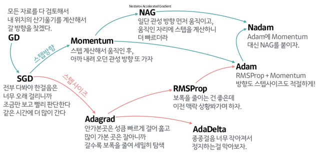
그림으로 보는 다양한 최적화 기법들도 참조하세요.
가중치의 초기값
가중치의 초깃값을 무엇으로 설정하느냐에 따라 신경망 학습의 성패가 갈라지기도 합니다. 이번 절에서는 권장 초깃값에 대해서 설명하고 실험을 통해 실제로 신경망 학습이 신속하게 이뤄지는 모습을 확인해봅니다.
초깃값을 0으로 하면?
지금까지 가중치의 초깃값은 0.01 * np.random.randn(10, 100) 처럼 정규분포에서 생성되는 값을 사용했습니다.
초깃값을 모두 0으로 해서는 안되는 이유(정확히는 가중치를 균일한 값으로 설정해서는 안되는 이유)는 오차역전파법에서 모든 가중치의 값이 똑같이 갱신되기 때문입니다.
예를 들어 2층 신경망에서 첫 번째와 두 번째 층의 가중치가 0이라고 가정합니다. 그러면 순전파 때는 입력층의 가중치가 0이기 때문에 두 번째 층의 뉴런에 모두 같은 값이 전달됩니다. 두 번째 층의 모든 뉴런에 같은 값이 입력된다는 것은 역전파 때 두 번째 층의 가중치가 모두 똑같이 갱신된다는 말이 됩니다. 그래서 가중치들은 같은 초깃값에서 시작하고 갱신을 거쳐도 여전히 같은 값을 유지합니다. 이는 가중치를 여러 개 갖는 의미를 사라지게 합니다. 이렇게 가중치가 고르게 되어버리는 상황을 막으려면 초깃값을 무작위로 설정해야 합니다.
은닉층의 활성화값 분포
 1def sigmoid(x):
 2    return 1 / (1 + np.exp(-x))
 3
 4input_data = np.random.randn(1000, 100)  # 1000개의 데이터
 5node_num = 100  # 각 은닉층의 노드(뉴런) 수
 6hidden_layer_size = 5  # 은닉층이 5개
 7activations = {}  # 이곳에 활성화 결과를 저장
 8
 9x = input_data
10
11for i in range(hidden_layer_size):
12    if i != 0:
13        x = activations[i-1]
14
15    # 초깃값을 다양하게 바꿔가며 실험해보자!
16    w = np.random.randn(node_num, node_num) * 1
17    # w = np.random.randn(node_num, node_num) * 0.01
18    # w = np.random.randn(node_num, node_num) * np.sqrt(1.0 / node_num)
19    # w = np.random.randn(node_num, node_num) * np.sqrt(2.0 / node_num)
20
21
22    a = np.dot(x, w)
23
24
25    # 활성화 함수도 바꿔가며 실험해보자!
26    z = sigmoid(a)
27    # z = ReLU(a)
28    # z = tanh(a)
29
30    activations[i] = z
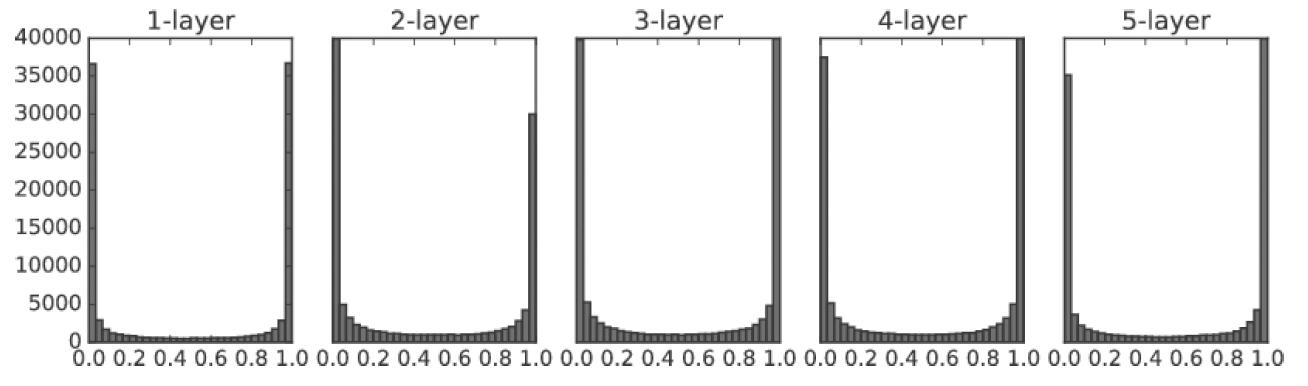
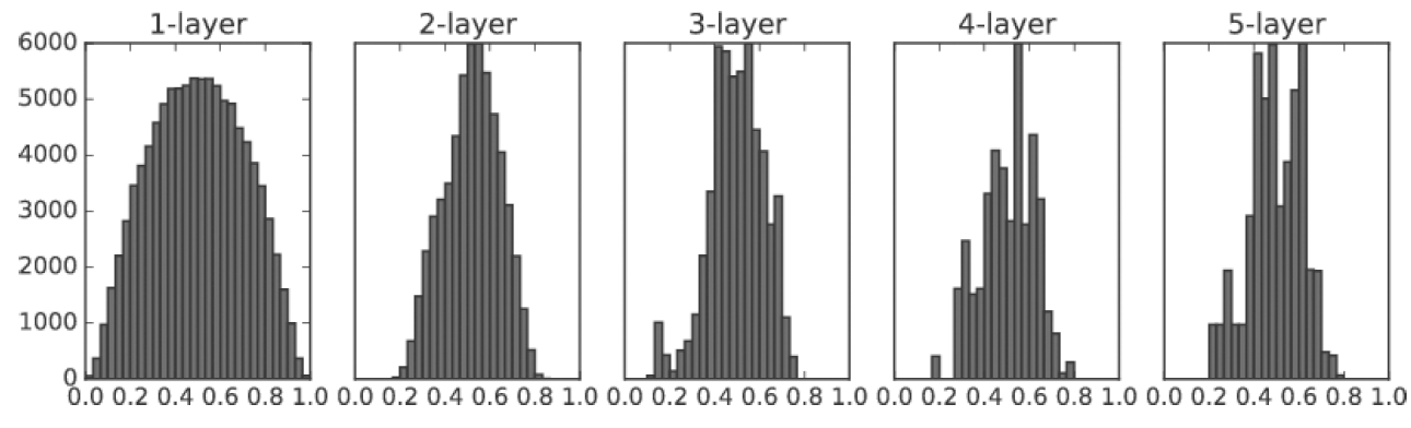
가중치 표준편차가 1인 정규분포로 초기화할 때의 각 층의 활성화값 분포
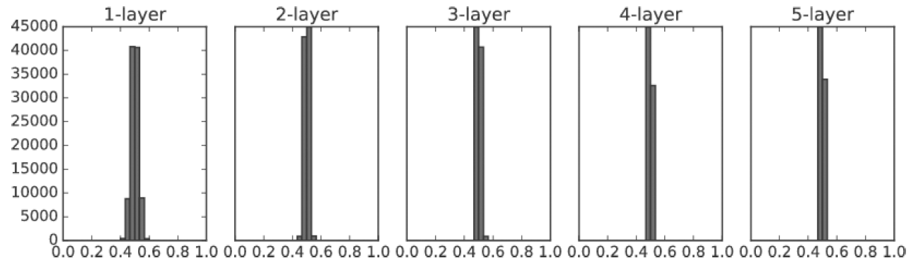
가중치 표준편차가 0.01인 정규분포로 초기화할 때의 각 층의 활성화값 분포
Xavier 8
Xavier 초기값
가중치 초기값으로 Xavier 초기값을 이용할 떄의 각 층의 활성화값 분포
ReLU를 사용할 때의 가중치 초기값
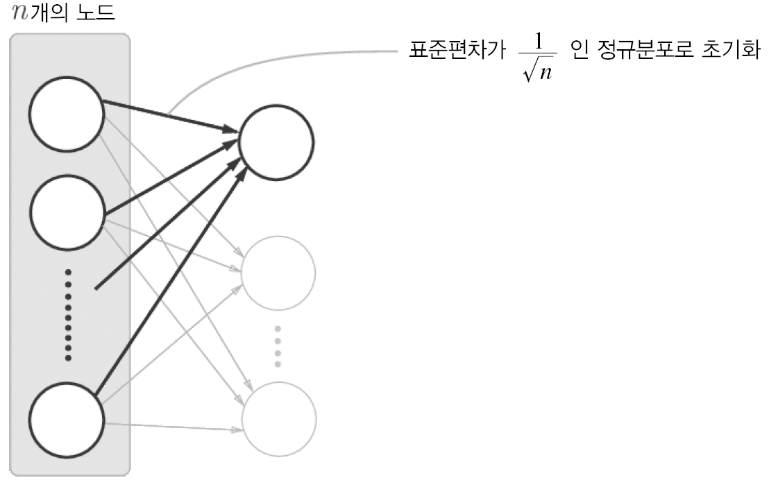
Relu를 이용할 때는 카이밍 히 Kaiming He의 이름을 딴 He 초기값이 권장됩니다. 6 He 초기값은 앞 계층의 노드가 \(n\) 개일 때 표준편차가 \(\sqrt{\dfrac{2}{n}}\)인 정규분포를 이용합니다.
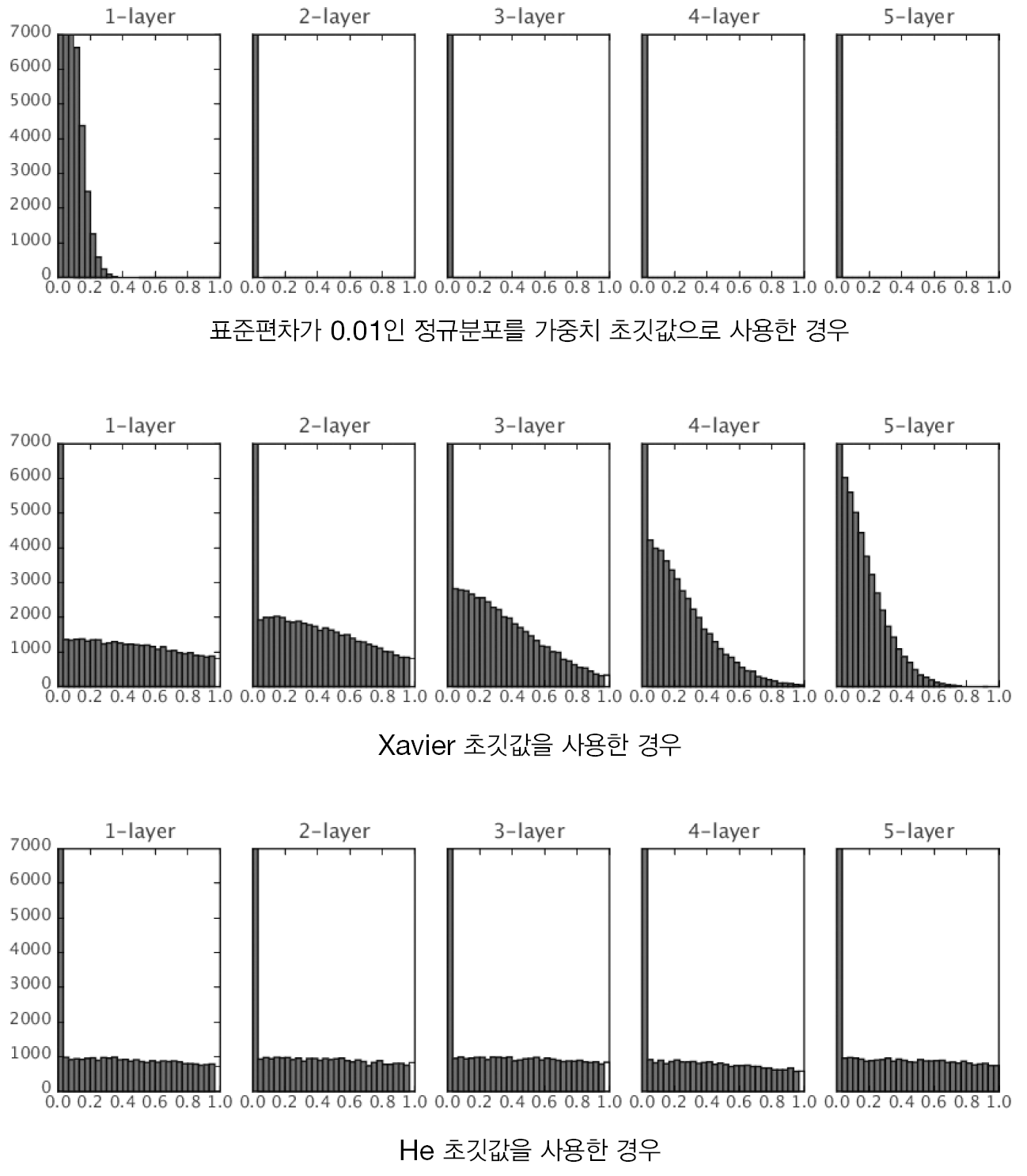
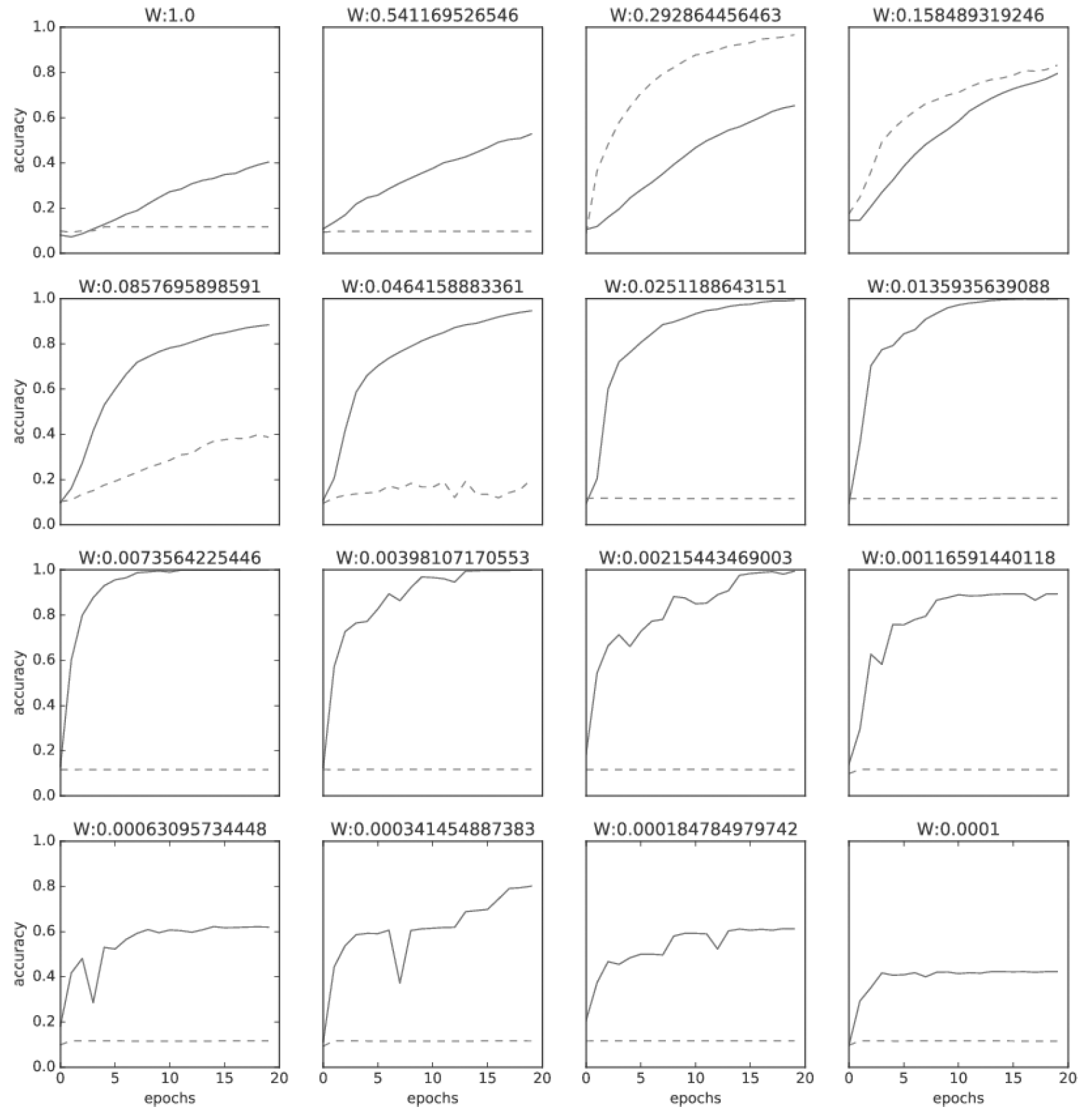
활성화 함수로 ReLU를 사용한 경우의 가중치 초깃값 변화에 따른 활성화값 분포 변화
MNIST 데이터셋으로 본 가중치 초깃값 비교
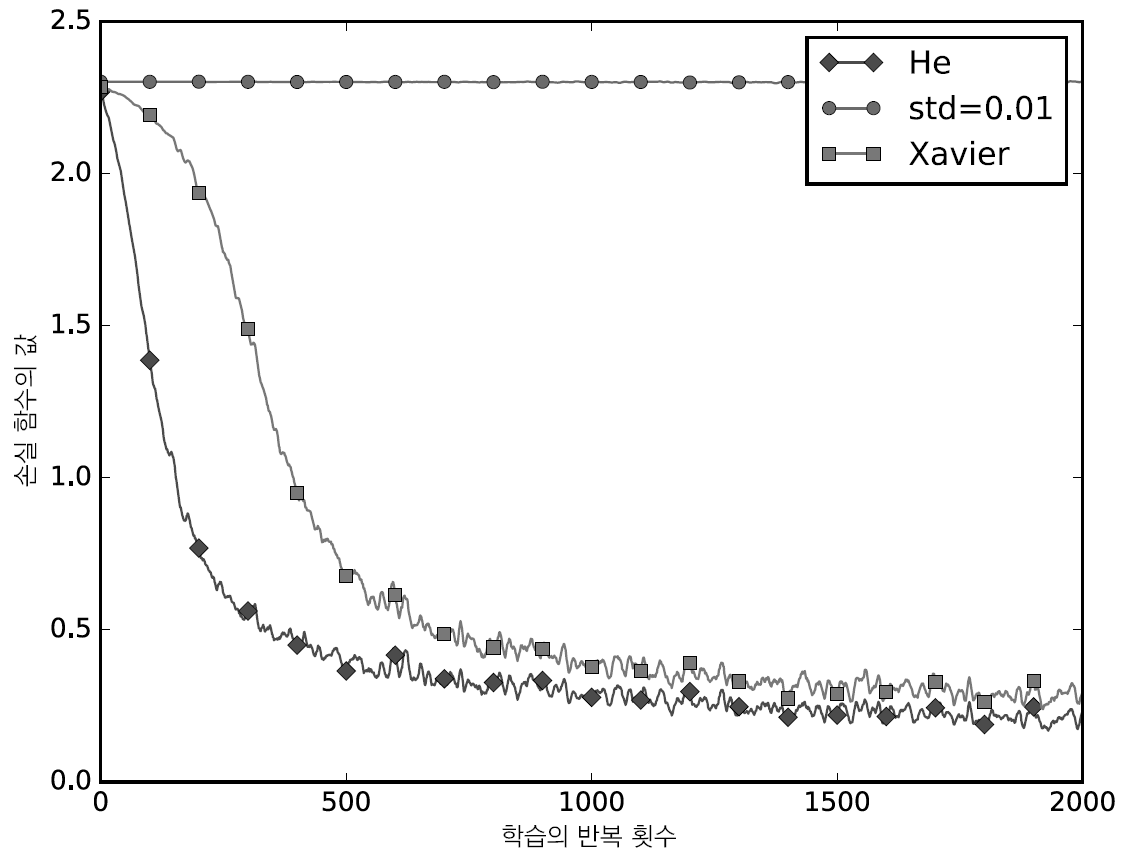
MNIST 데이터셋으로 살펴본 가중치 초깃값 비교
 1# 0. MNIST 데이터 읽기==========
 2(x_train, t_train), (x_test, t_test) = load_mnist(normalize=True)
 3
 4train_size = x_train.shape[0]
 5batch_size = 128
 6max_iterations = 2000
 7
 8
 9# 1. 실험용 설정==========
10weight_init_types = {'std=0.01': 0.01, 'Xavier': 'sigmoid', 'He': 'relu'}
11optimizer = SGD(lr=0.01)
12
13networks = {}
14train_loss = {}
15for key, weight_type in weight_init_types.items():
16    networks[key] = MultiLayerNet(input_size=784, hidden_size_list=[100, 100, 100, 100],
17                                  output_size=10, weight_init_std=weight_type)
18    train_loss[key] = []
19
20
21# 2. 훈련 시작==========
22for i in range(max_iterations):
23    batch_mask = np.random.choice(train_size, batch_size)
24    x_batch = x_train[batch_mask]
25    t_batch = t_train[batch_mask]
26
27    for key in weight_init_types.keys():
28        grads = networks[key].gradient(x_batch, t_batch)
29        optimizer.update(networks[key].params, grads)
30
31        loss = networks[key].loss(x_batch, t_batch)
32        train_loss[key].append(loss)
33
34    if i % 100 == 0:
35        print("===========" + "iteration:" + str(i) + "===========")
36        for key in weight_init_types.keys():
37            loss = networks[key].loss(x_batch, t_batch)
38            print(key + ":" + str(loss))
 1class MultiLayerNet:
 2    """완전연결 다층 신경망
 3
 4    Parameters
 5    ----------
 6    input_size : 입력 크기(MNIST의 경우엔 784)
 7    hidden_size_list : 각 은닉층의 뉴런 수를 담은 리스트(e.g. [100, 100, 100])
 8    output_size : 출력 크기(MNIST의 경우엔 10)
 9    activation : 활성화 함수 - 'relu' 혹은 'sigmoid'
10    weight_init_std : 가중치의 표준편차 지정(e.g. 0.01)
11        'relu'나 'he'로 지정하면 'He 초깃값'으로 설정
12        'sigmoid'나 'xavier'로 지정하면 'Xavier 초깃값'으로 설정
13    weight_decay_lambda : 가중치 감소(L2 법칙)의 세기
14    """
15    def __init__(self, input_size, hidden_size_list, output_size,
16                 activation='relu', weight_init_std='relu', weight_decay_lambda=0):
17        self.input_size = input_size
18        self.output_size = output_size
19        self.hidden_size_list = hidden_size_list
20        self.hidden_layer_num = len(hidden_size_list)
21        self.weight_decay_lambda = weight_decay_lambda
22        self.params = {}
23
24        # 가중치 초기화
25        self.__init_weight(weight_init_std)
26
27        # 계층 생성
28        activation_layer = {'sigmoid': Sigmoid, 'relu': Relu}
29        self.layers = OrderedDict()
30        for idx in range(1, self.hidden_layer_num+1):
31            self.layers['Affine' + str(idx)] = Affine(self.params['W' + str(idx)],
32                                                      self.params['b' + str(idx)])
33            self.layers['Activation_function' + str(idx)] = activation_layer[activation]()
34
35        idx = self.hidden_layer_num + 1
36        self.layers['Affine' + str(idx)] = Affine(self.params['W' + str(idx)],
37            self.params['b' + str(idx)])
38
39        self.last_layer = SoftmaxWithLoss()
40
41    def __init_weight(self, weight_init_std):
42        """가중치 초기화
43
44        Parameters
45        ----------
46        weight_init_std : 가중치의 표준편차 지정(e.g. 0.01)
47            'relu'나 'he'로 지정하면 'He 초깃값'으로 설정
48            'sigmoid'나 'xavier'로 지정하면 'Xavier 초깃값'으로 설정
49        """
50        all_size_list = [self.input_size] + self.hidden_size_list + [self.output_size]
51        for idx in range(1, len(all_size_list)):
52            scale = weight_init_std
53            if str(weight_init_std).lower() in ('relu', 'he'):
54                scale = np.sqrt(2.0 / all_size_list[idx - 1])  # ReLU를 사용할 때의 권장 초깃값
55            elif str(weight_init_std).lower() in ('sigmoid', 'xavier'):
56                scale = np.sqrt(1.0 / all_size_list[idx - 1])  # sigmoid를 사용할 때의 권장 초깃값
57            self.params['W' + str(idx)] = scale * np.random.randn(all_size_list[idx-1], all_size_list[idx])
58            self.params['b' + str(idx)] = np.zeros(all_size_list[idx])
배치 정규화
배치 정규화는 각 층의 활성화 값이 적당히 분포되도록 조정하는 아이디어로부터 출발합니다.
배치 정규화 알고리즘
배치 정규화가 주목받는 이유는 다음과 같습니다.
학습을 빨리 진행할 수 있습니다.
초깃값에 크게 의존하지 않습니다.
오버피팅 overfitting을 억제 합니다.
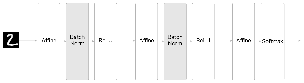
배치 정규화를 사용한 신경망의 예
배치 정규화는 학습 시 미니배치를 단위로 정규화합니다. 구체적으로 데이터 분포가 평균이 0, 분산이 1이 되도록 정규화합니다. 수식은 다음과 같습니다.
여기서 \(B\)는 \(m\) 개의 입력데이터 \(\{x_1, x_2, \ldots, x_m \}\)를 의미하고, \(B\)에 대한 평균 \(\mu_B\) 와 분산 \(\sigma_B^2\)을 구합니다.
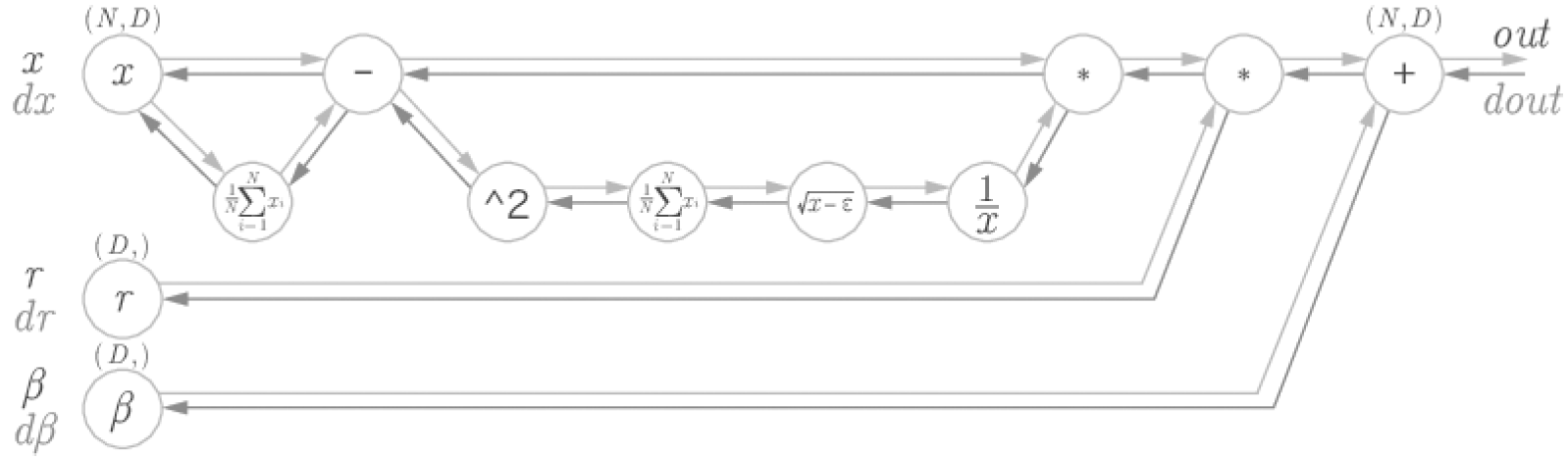
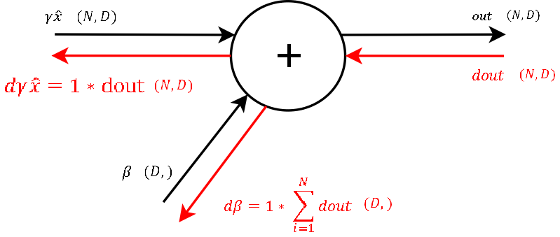
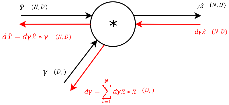
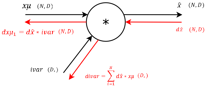
배치 정규화의 계산 그래프
배치 정규화 역전파 그래프는 프레드릭 크레저트 Frederick Kratzert의 블로그 7를 참고하세요.
Step 9(출처: Understanding the backward pass through Batch Normalization Layer)
Step 8(출처: Understanding the backward pass through Batch Normalization Layer)
Step 7(출처: Understanding the backward pass through Batch Normalization Layer)
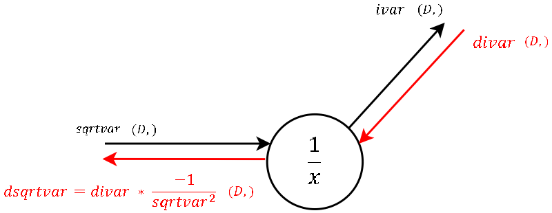
Step 6(출처: Understanding the backward pass through Batch Normalization Layer)
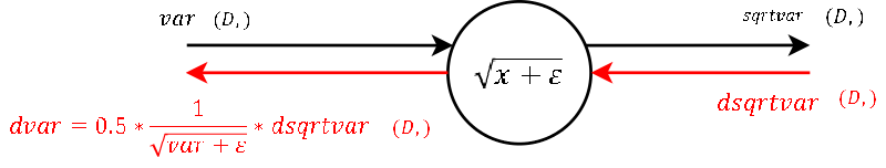
Step 5(출처: Understanding the backward pass through Batch Normalization Layer)
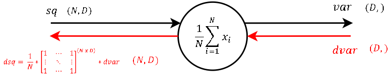
Step 4(출처: Understanding the backward pass through Batch Normalization Layer)
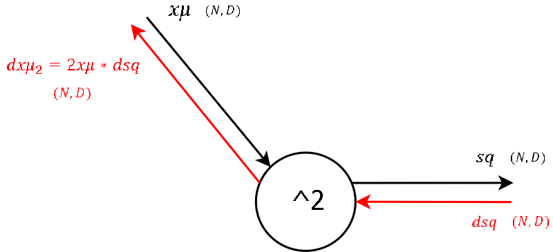
Step 3(출처: Understanding the backward pass through Batch Normalization Layer)
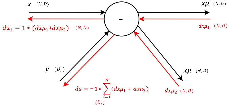
Step 2(출처: Understanding the backward pass through Batch Normalization Layer)
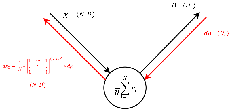
Step 1(출처: Understanding the backward pass through Batch Normalization Layer)
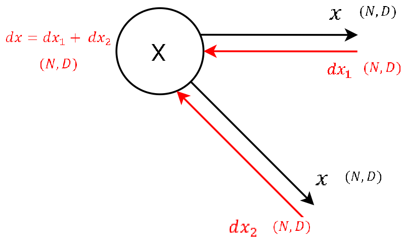
Step 0(출처: Understanding the backward pass through Batch Normalization Layer)
배치 정규화의 효과
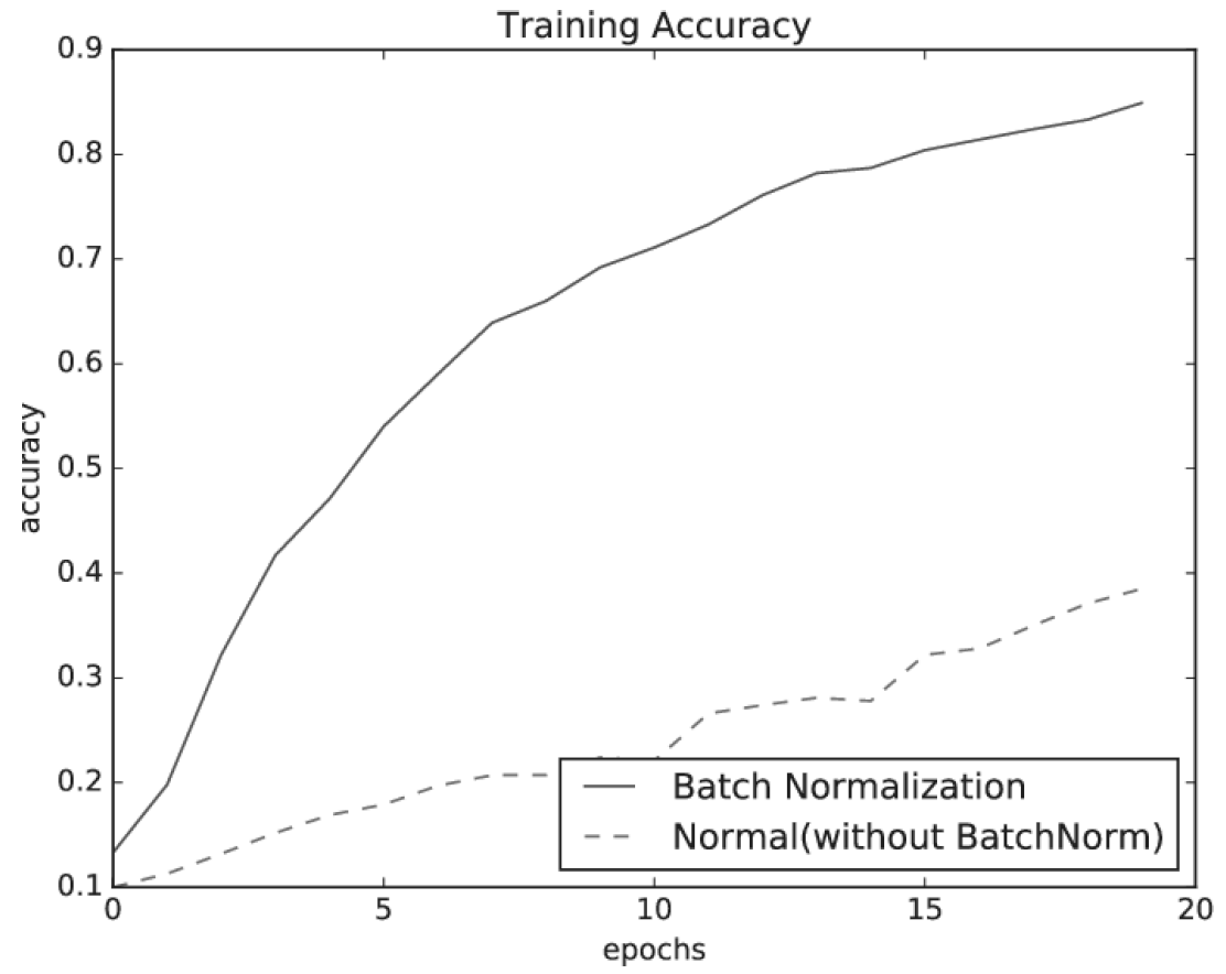
배치 정규화의 효과
가중치 초깃값의 변경
바른 학습을 위해
오버피팅
가중치 감소
드롭아웃 Dropout
드롭아웃은 뉴런을 임의로 삭제하면서 학습하는 방법입니다. 5 학습할 때 은닉층의 뉴런을 무작위로 골라 삭제하기 때문에 삭제된 뉴런은 신호를 전달하지 않게 됩니다. 학습할 때는 데이터가 입력될 때마다 삭제할 뉴런을 무작위로 선택하고, 시험 때는 모든 뉴런에 신호를 전달합니다. 단, 시험 때는 각 뉴런의 출력에 학습 때 삭제 안한 비율을 곱하여 출력합니다.
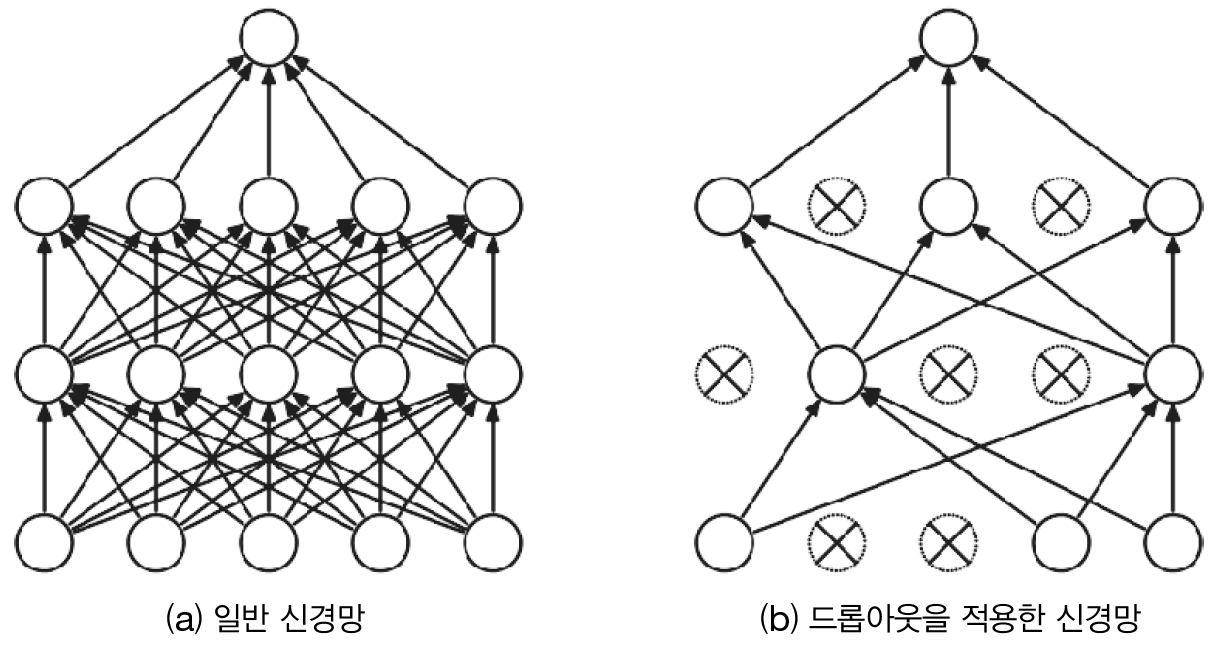
드롭아웃 개념
Dropout 클래스 1class Dropout:
2 """
3 http://arxiv.org/abs/1207.0580
4 """
5 def __init__(self, dropout_ratio=0.5):
6 self.dropout_ratio = dropout_ratio
7 self.mask = None
8
9 def forward(self, x, train_flg=True):
10 if train_flg:
11 self.mask = np.random.rand(*x.shape) > self.dropout_ratio
12 return x * self.mask
13 else:
14 return x * (1.0 - self.dropout_ratio)
15
16 def backward(self, dout):
17 return dout * self.mask
11-12줄:
np.random.rand는 uniform 분포를 따르는 무작위 수를 반환하므로self.dropout_ratio보다 큰 뉴런들만 반환합니다.14줄: 시험 데이터(
train_flg=False) 또는 정확도를 측정할 때는 삭제 안한 비율을 곱하여 반환합니다. 517줄: 역전파할 때도 순전파할 때 사용되었던 값 들에대해서만 흘려 보냅니다.
드롭아웃 효과를 MNIST 데이터셋을 이용해 확인해 봅니다.
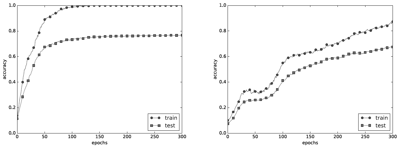
왼쪽은 드롭아웃 없이, 오른쪽은 드롭아웃을 적용한 결과(dropout_ratio=0.15)
드롭아웃 실험은 7층(각 층의 뉴런 수는 100개, 활성화 함수는 Relu)의 네트워크를 써서 진행합니다.
Affine -> Dropout -> Affine -> Dropout -> Affine -> Dropout -> Affine -> Dropout -> Affine -> Dropout -> Affine -> Dropout -> Affine -> SoftmaxWithLoss
그림과 같이 드롭아웃을 적용할 때는 훈련데이터와 시험데이터에 대한 각 에폭에서 정확도 차이가 줄어든 것을 알 수 있습니다.
다음은 위 실험에 관한 코드입니다.
 1from dataset.mnist import load_mnist
 2from common.multi_layer_net_extend import MultiLayerNetExtend
 3from common.trainer import Trainer
 4
 5(x_train, t_train), (x_test, t_test) = load_mnist(normalize=True)
 6
 7# 오버피팅을 재현하기 위해 학습 데이터 수를 줄임
 8x_train = x_train[:300]
 9t_train = t_train[:300]
10
11# 드롭아웃 사용 유무와 비울 설정 ========================
12use_dropout = True  # 드롭아웃을 쓰지 않을 때는 False
13dropout_ratio = 0.2
14# ====================================================
15
16network = MultiLayerNetExtend(input_size=784, hidden_size_list=[100, 100, 100, 100, 100, 100],
17                              output_size=10, use_dropout=use_dropout, dropout_ration=dropout_ratio)
18trainer = Trainer(network, x_train, t_train, x_test, t_test,
19                  epochs=301, mini_batch_size=100,
20                  optimizer='sgd', optimizer_param={'lr': 0.01}, verbose=True)
21trainer.train()
22
23train_acc_list, test_acc_list = trainer.train_acc_list, trainer.test_acc_list
24
25# 그래프 그리기==========
26markers = {'train': 'o', 'test': 's'}
27x = np.arange(len(train_acc_list))
28plt.plot(x, train_acc_list, marker='o', label='train', markevery=10)
29plt.plot(x, test_acc_list, marker='s', label='test', markevery=10)
30plt.xlabel("epochs")
31plt.ylabel("accuracy")
32plt.ylim(0, 1.0)
33plt.legend(loc='lower right')
34plt.show()
12줄:
use_dropout값에 따라 결과가 다르게 나옵니다.16-17줄: 은닉층
hidden_size_list이 6개, 출력층output_size1개 총 7개의 계층으로 구성됩니다.19줄: 300 에폭을 실행합니다.